Bitcoin's Power Law: the equation that predicts price with R² = 0.96
How I built an interactive dashboard that fits 15 years of Bitcoin prices to a power law, decomposes cycles with Fourier analysis, and estimates the next peak. Real math, no financial astrology.
R² = 0.9668
That’s the goodness of fit for a model that predicts Bitcoin’s price using a single equation:
price = coefficient × days^exponentFifteen years of data. From $0.01 in 2009 to the $69,000 peaks. A power law explains 96.68% of the price variance.
The model doesn’t predict tomorrow. It predicts the trajectory — a channel within which Bitcoin moves, with statistical floors and ceilings that historically coincide with each cycle’s bottoms and bubbles.
I built an interactive dashboard to visualize all of this. It runs in the browser, has no backend, and pulls data from CoinGecko. It’s live at juanarnaboldi.com.ar/power-law-bitcoin.
What a power law is
A power law describes a relationship where one quantity varies as a power of another. On a log-log scale, a power law is a straight line.
Bitcoin grows as a power law — not exponential, not linear. Each order of magnitude takes longer than the last. The jump from $1 to $10 was fast. From $10,000 to $100,000 takes years.
The hypothesis comes from physicist Giovanni Santostasi, who in 2014 noticed that plotting Bitcoin’s price on a log-log scale against days since the genesis block produces points that align on a straight line with absurd consistency.
Why a power law? Power laws emerge in complex systems with positive feedback: city growth, earthquake distribution, social networks. Bitcoin has an explicit feedback mechanism: the halving cuts emissions every 210,000 blocks (~4 years), creating scarcity cycles that fuel demand.
The regression: OLS in log-log space
The model is ordinary least squares regression, applied to the logarithms:
log₁₀(price) = log₁₀(coefficient) + exponent × log₁₀(days)You transform a power curve into a straight line. Fit with least squares. Transform back.
export function powerLawRegression(data: [number, number][]): PowerLawResult {
  const points: [number, number][] = [];
  for (const [ts, price] of data) {
    const days = (ts - GENESIS_MS) / MS_PER_DAY;
    if (days > 200 && price > 0) {
      points.push([Math.log10(days), Math.log10(price)]);
    }
  }

  const n = points.length;
  let sx = 0,
    sy = 0,
    sxy = 0,
    sxx = 0;
  for (const [x, y] of points) {
    sx += x;
    sy += y;
    sxy += x * y;
    sxx += x * x;
  }

  const exponent = (n * sxy - sx * sy) / (n * sxx - sx * sx);
  const intercept = (sy - exponent * sx) / n;
  const coefficient = Math.pow(10, intercept);

  // R² and sigma
  const yMean = sy / n;
  let ssTot = 0,
    ssRes = 0;
  for (const [x, y] of points) {
    const yHat = exponent * x + intercept;
    ssTot += (y - yMean) ** 2;
    ssRes += (y - yHat) ** 2;
  }

  return {
    exponent,
    coefficient,
    rSquared: 1 - ssRes / ssTot,
    sigma: Math.sqrt(ssRes / (n - 2)),
  };
}
The days > 200 filter discards the first months when Bitcoin was traded between a handful of people at sub-penny prices. That’s noise from a nonexistent market.
The result: an exponent of ~5.6, a coefficient of ~5.5×10⁻¹⁷, and a sigma of ~0.28. Sigma defines the support (-2σ) and resistance (+2σ) bands around fair value.
Residuals and Z-Score: cheap or expensive?
The residual measures how far the current price deviates from the model’s predicted fair value:
residual = log₁₀(actual_price) - log₁₀(model_price)
z_score = residual / sigma
A Z-Score of -0.92 means the price is 0.92 standard deviations below fair value. Historically, 83.5% of the time it was more expensive than now.
Bubble peaks coincide with extreme Z-Scores. November 2021 ($69K) hit a Z-Score of ~+1.5. Bear market bottoms drop below -1.5.
The historical percentile adds context: it tells you where the current price sits relative to the entire model history. A 16.5% percentile means 83.5% of recorded days saw Bitcoin priced higher in relative terms.
Fourier: taking the cycles apart
The residuals aren’t random noise. They have periodicity. Apply a Fast Fourier Transform (FFT) and the signal decomposes into sinusoidal components with defined frequencies, amplitudes, and phases.
The implementation uses the Cooley-Tukey radix-2 algorithm — the classic FFT with bit-reversal permutation and butterfly operations:
export function fft(re: Float64Array, im: Float64Array): void {
  const n = re.length;
  // Bit-reversal permutation
  for (let i = 1, j = 0; i < n; i++) {
    let bit = n >> 1;
    for (; j & bit; bit >>= 1) j ^= bit;
    j ^= bit;
    if (i < j) {
      [re[i], re[j]] = [re[j], re[i]];
      [im[i], im[j]] = [im[j], im[i]];
    }
  }
  // Butterfly operations
  for (let len = 2; len <= n; len *= 2) {
    const angle = (-2 * Math.PI) / len;
    const wRe = Math.cos(angle);
    const wIm = Math.sin(angle);
    for (let i = 0; i < n; i += len) {
      let curRe = 1,
        curIm = 0;
      for (let j = 0; j < len / 2; j++) {
        const k = i + j + len / 2;
        const tRe = curRe * re[k] - curIm * im[k];
        const tIm = curRe * im[k] + curIm * re[k];
        re[k] = re[i + j] - tRe;
        im[k] = im[i + j] - tIm;
        re[i + j] += tRe;
        im[i + j] += tIm;
        const newCurRe = curRe * wRe - curIm * wIm;
        curIm = curRe * wIm + curIm * wRe;
        curRe = newCurRe;
      }
    }
  }
}
From all the frequencies the FFT extracts, the system sorts by amplitude and takes the top 8. The fundamental has a period of ~6.3 years. The first harmonic falls at ~4.7 years — suspiciously close to the halving cycle (~4 years).
Each component has frequency, amplitude, and phase. With those three parameters you can reconstruct the original signal and — more interesting — extrapolate into the future:
export function forecastSignal(
  frequencies: FrequencyComponent[],
  startIndex: number,
  forecastLength: number,
  sampleIntervalDays: number,
  activeIndices?: Set<number>
): number[] {
  const signal = new Array<number>(forecastLength).fill(0);
  for (const comp of frequencies) {
    if (activeIndices && !activeIndices.has(comp.index)) continue;
    for (let t = 0; t < forecastLength; t++) {
      const days = (startIndex + t) * sampleIntervalDays;
      signal[t] += comp.amplitude * Math.cos(2 * Math.PI * comp.frequency * days + comp.phase);
    }
  }
  return signal;
}
The forecast extends 730 days ahead. The dashboard lets you toggle individual harmonics to see how each one contributes to the reconstructed signal’s shape.
Market phases
With the reconstructed signal and its derivative, the system automatically classifies the market phase:
| Phase | Signal | Derivative | Meaning |
|---|---|---|---|
| Accumulation | < 0 | > 0 | Low price, starting to rise |
| Bull | ≥ 0 | > 0 | High price, still rising |
| Distribution | ≥ 0 | ≤ 0 | High price, starting to fall |
| Bear | < 0 | ≤ 0 | Low price, still falling |
export function detectPhase(signalValue: number, derivative: number): MarketPhase {
  if (signalValue < 0 && derivative > 0) return 'acumulación';
  if (signalValue >= 0 && derivative > 0) return 'alcista';
  if (signalValue >= 0 && derivative <= 0) return 'distribución';
  return 'bajista';
}
It’s a four-quadrant classifier based on the Fourier signal’s position and momentum. Nothing sophisticated, but the combination with Z-Score produces trading signals that are surprisingly coherent with history.
The trading signal
Everything converges into a function that combines Z-Score and market phase to produce BUY, SELL, or HOLD with a confidence percentage:
export function computeSignal(zScore: number, phase: MarketPhase): TradingSignal {
  if (zScore < -1.5)
    return {
      type: 'COMPRA',
      confidence: 95,
      reason: 'Extremely low Z-Score: price far below fair value',
    };
  if (zScore > 1.5)
    return {
      type: 'VENTA',
      confidence: 95,
      reason: 'Extremely high Z-Score: price far above fair value',
    };
  if (zScore < 0 && (phase === 'acumulación' || phase === 'alcista')) {
    const conf = phase === 'acumulación' ? 70 : 60;
    return { type: 'COMPRA', confidence: conf, reason: `Price below fair value in ${phase} phase` };
  }
  // ... more rules for SELL and HOLD
  return { type: 'HOLD', confidence: 50, reason: 'No clear signal' };
}
Extremes (±1.5σ) give 95% confidence. These are rare events — bubble peaks and absolute bear market bottoms. In between, the market phase modulates confidence: a negative Z-Score during accumulation is more convincing than during distribution.
The stack
React 19 + TypeScript + Vite 8
├── Canvas API              → main log-log chart (pixel-perfect)
├── Lightweight Charts 5    → residuals and Fourier (interactive)
├── CoinGecko API           → live prices (every 60s)
├── Historical data         → bundled from January 2009
└── Tailwind CSS            → dark terminal-style UI
Architecture decisions that matter:
Native Canvas for the main chart. Lightweight Charts doesn’t support dual log-log scales. The Power Law chart needs to map coordinates in logarithmic space on both axes, with interactive zoom, tooltips, and annotations for halvings and bubble peaks. Canvas is the only option that gives the necessary control.
Lightweight Charts for secondary panels. Residuals and Fourier are conventional time series. Lightweight Charts handles zoom, crosshair, and responsiveness for free.
No backend. All the math runs in the browser. Historical data (2009-present) is bundled in a 1,431-line file. The last 365 days refresh from CoinGecko every 5 minutes. Current price updates every 60 seconds.
A single useMemo. The entire analysis — regression, residuals, FFT, reconstruction, phases, signal, peak estimation — is computed in a memoized hook that depends on three variables: data, current price, and active harmonics. React doesn’t recalculate anything until something changes.
What the model says today
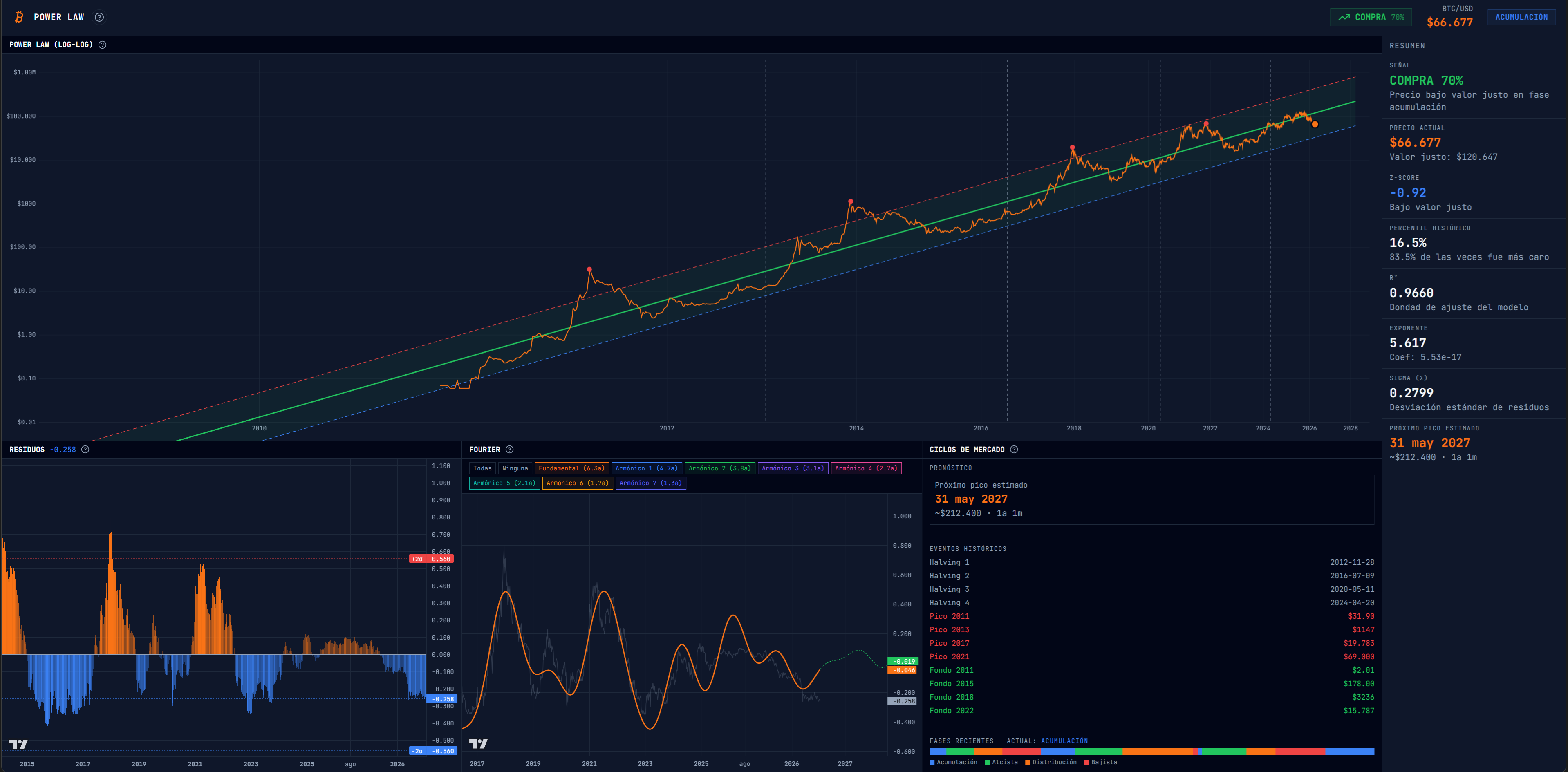
The dashboard shows in real time:
- Signal: BUY 70% — price below fair value in accumulation phase
- Current price: $66,677
- Fair value: $128,647
- Z-Score: -0.92 — below fair value
- Historical percentile: 16.5% — 83.5% of the time it was more expensive
- Estimated next peak: May 31, 2027, ~$212,400
These numbers update every time a new price comes in from CoinGecko.
What the model can’t tell you
Exact timing. The Fourier forecast estimates windows of months, not days. “May 2027” could be March or September.
Black swans. Regulations, exchange hacks, or a global recession aren’t in the historical residuals. The model assumes the future resembles the past — until it doesn’t.
The end of the pattern. A power law with R² = 0.96 over 15 years is impressive, but there’s no guarantee it continues. Bitcoin could saturate, adoption could stall, or a competitor could change the dynamics. The model describes what happened, it doesn’t promise what will.
Financial advice. This is a quantitative analysis tool built as a personal project. The signals are the output of a mathematical equation, not a certified analyst’s opinion.
The point
The math behind Bitcoin is more interesting than the speculation. A log-log regression, an FFT on the residuals, and a phase classifier produces a model that explains 15 years of history with R² = 0.96 and estimates future cycles within a reasonable margin.
It all runs in the browser. ~200KB gzipped. No server, no database, no subscription.
The tool is live at juanarnaboldi.com.ar/power-law-bitcoin.